knitr::opts_chunk$set(cache = TRUE,
                      echo = TRUE,
                      message = FALSE,
                      warning = FALSE,
                      fig.path = "static",
                      fig.height=6,
                      fig.width = 1.777777*6,
                      fig.align='center',
                      tidy = FALSE,
                      comment = NA,
                      highlight = TRUE,
                      prompt = FALSE,
                      crop = TRUE,
                      comment = "#>",
                      collapse = TRUE)
knitr::opts_knit$set(width = 60)
library(tidyverse)
library(reshape2)
theme_set(theme_light(base_size = 16))
make_latex_decorator <- function(output, otherwise) {
  function() {
      if (knitr:::is_latex_output()) output else otherwise
  }
}
insert_pause <- make_latex_decorator(". . .", "\n")
insert_slide_break <- make_latex_decorator("----", "\n")
insert_inc_bullet <- make_latex_decorator("> *", "*")
insert_html_math <- make_latex_decorator("", "$$")Factors Affecting neonatal Mortality
survival analysis
clinical trials
GLMS
Introduction
Neonatals death refers to the death of newborns before they turn 28 days old (Usman et al.,2019), and can be categorized as early or late depending on whether the death occurred before or after the seventh day of life. The period after birth is widely regarded as the most vulnerable and high-risk time for newborns. This is due to the fact that mortality and morbidity rates are significantly elevated during this period. Studies indicate that over 50% of child deaths occur as early as the first two days of birth, while over 75% occur within the first week (Carlo & Travers, 2016). Some researchers argue that time with the highest chances of neonatal death is within the first 24 hours of life (Nouri et al., 2013). Globally, neonatal mortality accounts for about 44% of child mortality and over 60% of infant mortality, resulting in approximately 2.8 million deaths each year (UNICEF,2014).\
The objectives of the study are to:
General survival analysis ideas
Survival analysis deals with the study of time till a certain event of interest occurs.
Censoring
Censoring in survival analysis refers to the situation where the outcome(e.g., death, hospitalization, etc.) has not occurred for some subjects by the end of the study. This can occur for various reasons, such as loss to follow-up, withdrawal from the study, or the occurrence of another event that renders the subject no longer at risk for the event of interest. The common types of censoring include :
Because of censoring,we can not use the usual ordinay statistical methods because we can not compute the descriptive statistics like sample mean,standard deviation or even peform regression analysis.
Survival function
Survival analysis typically involves using T as the response variable, as it represents the time till an outcome occurs, while t refers to the actual survival time of an individual. The distribution function F(t) is used to describe chances of time of survival being less than a given value, t. In some cases, the cumulative distribution function is of interest and can be obtained as follows:
\[\begin{equation} F(t)=P(T\le t)=\int_{t}^{\infty}f(u) \end{equation}\] Interest also tends to focus on the survival or survivorship function which in this study is the chances of a neonate surviving after time \(t\) and also given by the formula
\[\begin{equation} S(t) = P(T > t)=\int_{t}^{\infty} f(u) du \end{equation}\]\(S(t)\) monotonically decreasing function with \(S(0) = 1\) and \(S(\infty) = \text{lim}_{t \rightarrow \infty} S(t) = 0\).
Suppose we have \(R (t)\) (set at risk) that has neonates who are prone to dying by time t, the chances of a neonate in that set to die in a given interval \([t, t + \delta t)\) is given by the following forrmula, where \(h(t)\) is the hazard rate and is defined as: \[\begin{equation} h(t) = \lim_{\delta t \rightarrow 0} \frac{P(t \le T < t+\delta t | T \ge t)}{\delta t} \end{equation}\] The hazard function’s shape can be any strictly positive function and it changes based on the specific survival data provided.
Relationship between h(t) and S(t)
It is given that \(f(t) = - \frac{d}{dt} S(t)\) hence the equation above can be simplified to:
\[\begin{equation} h(t)=\frac{f(t)}{S(t)} =\frac{- \frac{d}{dt} S(t)}{S(t)}= - \frac{d}{dt} [\log S(t)] \end{equation}\]Taking intergrals both sides the above reduces to: \[H(t)= -\log S(t)\]
where \(H(t)=\int_{t}^{t} h(u) du\) ,is the cumulative risk of a neonate dying by time t. Since the event is death, then H(t) summarises the risk of death up to time t, assuming that death has not occurred before t. The survival function is also approximately simplified as follows. [ S(t) = e^{-H(t)} -H(t) ]
Non-parametric methods
Estimates of the hazard and survival function are often used to summarize survival data and such methods are often referred to as Non-parametric methods of estimation. More detailed information such as the median and percentiles can be taken from the estimated survival function thereby giving more profound analysis (Cleves et al.,2008, Hanagal, 2011).
Empirical Survival Function
Assuming no censoring in the data points as well as no tied observations in the data. The empirical function of survival is used to give an estimate of S(t) in the absence of censoring and is given by:
\[\begin{align*} \hat{S}(t) = \frac{no~ of~neonates~ with~T \ge t} {total number of neonates} \end{align*}\]Kaplan-Meier estimate
If there are \(r\) times of deaths among neonates in ICU, such that \(r\leq n\) and \(n\) is the number of neonates with observed survival times. Arranging these times in from the smallest to the largest,the \(j\)-th death time is noted by \(t_{(j)}\) , for \(j = 1, 2, \cdots , r\), such that the \(r\) death times ordred are \[ t_{1}<t_{2}< \cdots < t_{m}\] . Let \(n_j\), for \(j = 1, 2, \ldots, r\), denote the number of neonates who are still alive before time \(t(j)\), including the ones that are expected to die at that time. Additionally, let \(d_j\) denote the number of neonates who die at time \(t(j)\). The estimate for the product limit can be expressed in the following form:
\[\begin{equation} \hat{S}(t) = \prod_{j=1}^k \, \left(1-\frac{d_j}{r_j}\right) \end{equation}\]To survive until time \(t\), a neonate must start by surviving till \(t(1)\), and then continue to survive until each subsequent time point \(t(2), \ldots, t(r)\). It is assumed that there are no deaths between two consecutive time points \(t(j-1)\) and \(t(j)\). The conditional probability of surviving at time \(t(i)\), given that the neonate has managed to survive up to \(t(i-1)\), is the complement of the proportion of the new born babies who die at time \(t(i)\), denoted by \(d_i\), to the new born babies who are alive just before \(t(i)\), denoted by \(n_i\). Therefore, the probability that is conditional of surviving at time \(t(i)\) is given by \(1 - \frac{d_i}{n_i}\). The variance of the estimator is given by \[\begin{equation} \text{var}(\hat{S}(t)) = [\hat{S}(t)]^2 \sum_{j=1}^k \frac{d_j}{(r_j-d_j) r_j} \end{equation}\] The corresponding standard deviation is therefore given by: \[\begin{equation} \text{s.e}(\hat{S}(t)) = [\hat{S}(t)]\left[\sum_{j=1}^k \frac{d_j}{(r_j-d_j) r_j}\right]^{\frac{1}{2}} \end{equation}\]
Log rank test
Given the problem of contrasting two or more survival functions,for instance survival times between male and female neonates in the ICU. Let \[ t_{1}<t_{2}< \cdots < t_{r}\]
Let \(t_i\) be the unique times of death observed among the neonates, found by joining all groups of interest. For group \(j\),\ let \(d_{ij}\) denote the number of deaths at time \(t_i\), and\ let \(n_{ij}\) denote the number at risk at time \(t_i\) in that group. Let \(d_i\) denote the total number of deaths at time \(t_i\) across all groups, and\
the expected number of deaths in group \(j\) at time \(t_i\) is: ,
\[E(d_{ij}) = \frac{n_{ij} \, d_i}{n_i} = n_{ij} \left(\frac{d_i}{n_i}\right) \]
At time \(t_i\), suppose there are \(d_i\) deaths and \(n_i\) individuals at risk in total, with \(d_{i0}\) and \(d_{i1}\) deaths and \(n_{i0}\) and \(n_{i1}\) individuals at risk in groups 0 and 1, respectively, such that \(d_{i0} + d_{i1} = d_i\) and \(n_{i0} + n_{i1} = n_i\). Such data can be summarized in a \(2 \times 2\) table at each death time \(t_i\).
Given that the null hypothesis is true, the number of deaths is expected to follow the hypergeometric distribution, and therefore: \[\begin{equation} E(d_{i0}) =e_{i0}= \frac{n_{i0} \, d_i}{n_i} = n_{i0} \left(\frac{d_i}{n_i}\right) \end{equation}\]
\[\begin{equation} \text{Var}(d_{i0}) = \frac{n_{i0} \, n_{i1} \, d_i(n_i-d_i)}{n_{i}^2 (n_{i}-1)} \end{equation}\] the statistic \(U_L\) is given by \[U_L=\sum^r_{i=1}(d_{i0}-e_{i0})\] so that the variance of \(U_L\) is \[Var(U_L)=\sum^r_{j=1}v_{i0}=V_L\] which then follows that : \[\frac{U_L}{\sqrt{V_L}} \sim N(0,1)\] and squaring results in \[\frac{U^2_L}{V_L}\sim \chi^2_1\]
Parametric survival distributions
Some of the most used parametric methods include the following:
Regression models in Survival analysis
Cox’s Proportional Hazards
The model is semi-parametric in nature since no assumption about a probabilty distribution is made for the survival times. The baseline model can take any form and the covariate enter the model linearly (Fox,2008). The model can thus be represented as :
\[\begin{equation} h(t|X) = h_0(t) \exp(\beta_1 X_{1} + \cdots + \beta_p X_{p})=h_0(t)\text{exp}^{(\beta^{T} X)} \end{equation}\]In the above equation, \(h_0(t)\) is known as the baseline hazard function, which represents the hazard function for a neonate when all the included variables in the model are zero. On the other hand, \(h(t|X)\) represents the hazard of a neonate at time \(t\) with a covariate vector \(X=(x_1,x_2,\ldots,x_p)\) and \(\beta^T=(\beta_1,\beta_2,\ldots,\beta_p)\) is a vector of regression coefficients.
Fitting a proportional hazards model
The partial likelihood
Given that \(t(1) < t(2) < \ldots < t(r)\) denote the \(r\) ordered death times. The partial likelihood is given by :
\[\begin{equation} L(\beta) = \prod_{i=1}^{n} \left[\frac{\text{exp}^{\beta ^{T} X_i}}{ \sum_{\ell\in R(t_{(i)}}\text{exp}^{\beta ^{T} X_\ell}}\right]^{\delta_i} \end{equation}\] Maximising the logarithmic of the likelihood function is more easier and computationally efficient and this is generally given by:
\[\begin{equation} \log L(\beta)= \sum_{i=1}^{n} \delta_i \left[ \beta ^{T} X_i - \log \left(\sum_{\ell \in R(t_{(i)}}\text{exp}^{\beta ^{T} X_\ell}\right) \right] \end{equation}\]Inference on the hazard ratios
Testing the conjecture that \(H_0 :\mathbf{\beta}=\mathbf{\beta_0}\) against \(H_a :\mathbf{\beta}\neq \mathbf{\beta_0}\) . Where \(\mathbf{\beta_0}\) is known,then
\[T=2 \left[\log(L(\hat{\mathbf{\beta}})) - \log(L(\mathbf{\beta_0}))\right]\] Where given the null hypothesis is true \(T\) has a of \(\chi^2_{(p)}\) and we can find the \(p\)-value at tail probablity of the \(\chi^2_{(p)}\) distribution as \(P(\chi^2_{(p)}\geq T)\)
The test statistic for the Wald test has a \(\chi^2\) distribution. To conduct a one-sided test at the \(\alpha\) level of significance, we compare the value of the test statistic, denoted as \(W\), to the chi-square value with \(1 - \alpha\) degrees of freedom.
\[\mathbf{\hat{\beta}} \sim N[\mathbf{\beta},I^{-1}(\mathbf{\hat{\beta}})]\]
According to Dobson (2002) ,the statistic
\[Z^{\*}_i=\frac{\hat{\beta_i}}{\text{s.e}(\hat{\beta_i})}\sim N(0,1)\] is called the wald statistic with a null hypthothesis \[H_0:\beta_i=0\]
Residuals for Cox Regression Model
Six types of residuals are studied in this thesis: Cox-Snell, Modified Cox-Snell, Schoenfeld, Martingale, Deviance, and Score residuals.
Cox-Snell ResidualS
Cox-Snell definition of residuals given by Cox and Snell (1968) is the most common residual in survival analysis. The Cox-Snell residual for the \(ith\) individual, \(i = 1, 2, \cdots , n\), is given by
\[\begin{equation} r_{Ci}=\text{exp}(\mathbf{\hat{\beta}^{T} x_i})\hat{H}_0(t_i) \end{equation}\] where \(\hat{H}_0(t_i)\) is an estimate of the baseline cumulative hazard function at time \(t_i\). It is sometimes called the Nelson-Aalen estimator.
Martingale residuals
These are useful in determing the functional form of the covariates to be included in the model. If the test reveals that the covariate can not be included linearly then there is need for such a covariate to be transformed . The martingale residuals are represented in the following form
\[\begin{equation} r_{Mi}=\delta_i - r_{Ci} \end{equation}\]Deviance Residuals
The skew range of Martingale residual makes it difficult to use it to detect outliers. The deviance residuals are much more symmetrically distributed about zero and are defined by \[\begin{equation} r_{Di}=\text{sgn}(r_{Mi})\left[-2\{r_{Mi}+\delta_i\log\left(\delta_i-r_{Mi}\right)\}\right]^{\frac{1}{2}} \end{equation}\]
Here, \(r_{Mi}\) represents the martingale residual for the \(i\)-th individual, and the function \(\text{sgn}(\cdot)\) denotes the sign function. Specifically, the function takes the value +1 if its argument is positive and -1 if negative.
Schoenfield residuals
Schoenfeld residuals are a useful tool for examining and testing the proportional hazard assumption, detecting leverage points, and identifying outliers. They can be calculated as follows: \[\begin{equation} r_{Sji}=\delta_i\{x_{ji}-\hat{a}_{ji}\} \end{equation}\] where \(x_{ji}\) is the value of the \(jth\) explanatory variable,\(j = 1, 2, \cdots , p\), for the \(ith\) individual in the study,
\[\begin{equation} \hat{a}_{ji}=\frac{\sum_{\ell \in R(t_i)}x_{j\ell}\text{exp}(\mathbf{\hat{\beta}^{T} x_{\ell}})}{\sum_{\ell \in R(t_i)}\text{exp}(\mathbf{\hat{\beta}^{T} x_{\ell}})} \end{equation}\]Parametric Proportional Hazard Models
The Cox regression model is often used in survival data analysis as it does not require a specific probability distribution assumption for the survival times. However, assuming a particular probability distribution can improve the precision of inferences, such as estimates of relative hazards and median survival times. Parametric models assume a specific probability distribution for the survival times.\
Weibull PH model
The hazard and the survival function of the Weibull distribution are given by,\ \(h(t) = \gamma \lambda t^{\gamma-1}\) and \(S(t) = e^{-\lambda t^\gamma}\) respectively. The hazard function of a neonate with covariates \(X_1,X_2,X_3,\cdots X_p\) is given by \[\begin{equation} h(t|X_i) =\gamma \lambda t^{\gamma-1} \exp(\beta_1 X_{i1} + \cdots + \beta_p X_{ip})=\gamma \lambda t^{\gamma-1}\text{exp}^{(\beta^{T} X)} \end{equation}\] making use of equation (\(\ref{cox}\)). The corresponding survival function is given by: \[\begin{equation} S_i(t)=\text{exp}\{\exp(\beta^{T} x_i)\lambda t^{\gamma}\} \end{equation}\] The model is filtted using the likelihood function of the \(n\) observations and maximizing this function with respect to unknown parameters \((\beta_1,\beta_2,\beta_3,\cdots,\beta_p),\lambda\) and \(\gamma\) where the likelihood function for the hazard and survivor function is given by : \[\begin{equation} L(\alpha,\mu,\sigma)=\prod_{i=1}^{n}\{h_i(t_i)\}^{\sigma_i}S_i(t_i) \end{equation}\] Taking logarithms in equation (\(\ref{parm}\)) we get \[\begin{equation} \log L(\alpha,\mu,\sigma)=\sum^{n}_{i=1}\{\sigma_i \log h_i(t_i)+\log S_i(t_i)\} \end{equation}\] Now substituting (\(\ref{gam}\)) and (\(\ref{parm}\)) and simplyfying we get \[\begin{equation} \log L(\alpha,\mu,\sigma)=\sum^n_{i=1}[\sigma_i\{\beta` x_i+\log(\lambda\gamma)+\gamma\log (t_i)\} -\lambda\text{exp}(\beta` x_i)t^{\gamma} \end{equation}\]
The Exponential PH model
The survival function and hazard function are given by \(S(t) = e^{-\lambda t}\) and \(h(t)=\sigma\) respectively. Evaluating equation (\(\ref{cox}\)) ,the hazard function for the exponential PH model of a particular neonate is given by
\[\begin{equation}
h(t|X_i) =\lambda \text{exp}(\beta_1 X_{i1} + \cdots + \beta_p X_{ip})=\lambda \text{exp}^{(\beta^{T} X)}
\end{equation}\]
Accelerated Failure Time Models
These models encompass a broader range of survival time distributions and may be more useful in situations where the proportional hazards assumption is not valid. Models based on this general family can prove to be fruitful. Under the accelerated failure time (AFT) models, we measure the direct impact of the explanatory variables on the survival time, instead of the hazard as we do in proportional hazards models. This approach facilitates the interpretation of results since the parameters quantify the impact of the corresponding covariate on the mean survival time. According to the general AFT model, the hazard function of the \(i\)-th neonate at time \(t\), \(h_i(t)\), is such that: \[\begin{equation}
h_i(t)=e^{-\phi_i}h_0(t/e^{-\phi_i})
\end{equation}\] The acceleration factor\(\phi_i\) is given according to the formula \[\phi_i =\text{exp}(\alpha_1x_{1i}+\alpha_2x_{2i}+ \cdots +\alpha_px_{pi}\] where \(x_{ji}\) is the value of the \(jth\) explanatory variable,\(X_j\),(\(j=1,2,3,\cdots,p\)),for the \(ith\) individual,(\(i=1,2,3,\cdots,n\)). For a group of neonates with with covariates \((X_1,X_2,\cdots,X_p)\),The survival function for the \(ith\) individual is given mathematically as \[\begin{equation}
S_i(t|x) = S_0(t/\phi_i)
\end{equation}\] Where \(S_0(t)\) is the baseline survival function and \(\phi\) is an accelerated factor implying a ratio of survival times corresponding to any fixed value of \(S(t)\). Parametric accelerated failure time models are unified by the adoption of a log-linear representation of the model and this form of the model is adopted by most computer software packages for accelerated failure time modelling. The log-linear model for the random variable \(T_i\) , associated with the lifetime of the \(ith\) individual in a survival study is given by
\[\begin{equation} \log T_i=\mu +\alpha_1x_{1i}+\alpha_2x_{2i}+ \cdots +\alpha_px_{pi}+\sigma\epsilon_i \end{equation}\] In this model, \(\alpha = (\alpha_1, \alpha_2, \ldots, \alpha_p)\) are the unknown coefficients of the explanatory variables \(X_1, X_2, \ldots, X_p\), with values \((x_{1i}, x_{2i}, \ldots, x_{pi})\) for the \(i\)-th individual. \(\mu\) and \(\sigma\) are two additional parameters known as the intercept and scale parameter, respectively. The quantity \(\sigma_i\) is a random variable used to model the deviation of the values of \(\log(T_i)\) from the linear component of the model. \(\sigma\) is a scale parameter and an error term typically expressed using a normal, logistic, or standard Gumbel distribution. The specific case of a standard Gumbel distribution for \(\sigma\) implies a conditional (on \(\beta\) and \(\sigma\)) Weibull survival model for \(T\) with shape parameter \(\alpha = 1/\alpha\) and scale parameter \(\lambda(\beta, \sigma) = \exp(-x^T\beta/\sigma)\) (Christensen et al., 2011). The \(\alpha\)-parameters reflect the impact of each explanatory variable on the survival times; positive values indicate that the survival time increases with increasing values of the explanatory variable, and vice versa. It can be shown that the survivor function for the \(i\)-th individual in an accelerated failure time model is given by: \[\begin{equation} S_i(t)=S_0\{t/\text{exp}(\alpha'x_i)\} \end{equation}\] The corresponding hazard function is also given by \[\begin{equation} h_i(t)=\text{exp}(\alpha'x_i)h_0\{t/\text{exp}(\alpha'x_i)\} \end{equation}\]
Weibull AFT model
Assuming that the survival times follow a Weibull distribution with scale parameter \(\lambda\) and shape parameter \(\gamma\) so that the baseline hazard as given by \(h(t) = \gamma \lambda t^{\gamma-1}\),the hazard function for the \(ith\) individual is then, from Equation (\(\ref{AFTS}\)), given by \[\begin{equation} h_i(t)=e^{-\phi_i}\lambda\gamma(e^{\phi_it})^{\gamma-1}=(e^{-\phi_i})^{\gamma}\lambda\gamma t^{\gamma-1} \end{equation}\] Implying that the survival time of the individual has a weibull distribution with scale parameter \(\lambda e^{-\gamma\phi_i}\) and shape parameter \(\gamma\). This property of the weibull distribution is called accelerated failure time property. The survivor and hazard function under the log-linear is given by
\[\begin{equation} S_i(t)=\text{exp}\left\{-\text{exp}\left(\frac{\log t -\mu -\phi_i}{\sigma}\right)\right\} \end{equation}\] and \[\begin{equation} h_i(t)=\frac{1}{\sigma t}\text{exp}\left(\frac{\log t -\mu -\phi_i}{\sigma}\right) \end{equation}\]
log-logistic AFT model
Suppose the suvival times follow a log-logistic distribution with a baseline hazard of \(h(t)=\frac{\exp^{\theta}kt^{k-1}}{1+\text{exp}^{\theta}t^k}\) ,it can be shown that the hazard function for the \(ith\) individual is then, from Equation (\(\ref{AFTS}\)), given by \[\begin{equation} h_i(t)=\frac{e^{\theta-k\phi_i}kt^{k-1}}{1+e^{\theta-k\phi_i}t^k} \end{equation}\] It then follows that the survival time for the ith individual also has a log-logistic distribution with parameters \(\theta- k\phi_i\) and \(k\). The log-linear form of the accelerated failure time model provides a representation of the log-logistic such that the survivor function of \(T_i\) is \[\begin{equation} S_i(t)=\left\{1+\text{exp}\left(\frac{\log t -\mu-\phi_i}{\sigma}\right)\right\}^{-1} \end{equation}\] where \(\phi_i=\alpha_1x_{1i}+\alpha_2x_{2i}+\cdots +\alpha_px_{pi}\) and corresponding hazard function given by \[\begin{equation} h_i(t)=\frac{1}{\sigma t}\left\{1+\text{exp}\left[-\left(\frac{\log t -\mu-\phi_i}{\sigma}\right)\right]\right\}^{-1} \end{equation}\]
Lognormal AFT model
The baseline survival function for a model that is assumed to have a logormal distribution is given below. survivor function is given by \[S_0(t)=1-\Phi\left(\frac{\log t- \mu}{\sigma}\right)\] The corresponding survivor function for the \(ith\) individual under the accelerated failure time model,is then \[S_i(t)=S_0(e^{-\phi_i}t)\] where \(\phi_i=\alpha_1x_{1i}+\alpha_2x_{2i}+\cdots +\alpha_px_{pi}\) is a linear combination of the values of \(p\) explanatory variables for the \(ith\) individual. This implies that the corresponding survivor function is given by \[\begin{equation} S_i(t) = 1- \Phi\left(\frac{\log t -\phi_i-\mu}{\sigma}\right) \end{equation}\] this is the survival function for an individual whose survival times have a lognormal distribution with parameters \(\mu +\phi_i\) and \(\sigma\). Implying that this model has the accelerated failure time property.
Model Checking
Akaike Information Criterion
Contrasting between a number of possible models, which can be unnested, can also be made on the basis of Akaike’s information criterion, given by \[AIC = -2logL + 2q\] in which \(q\) is the number of unknown \(\beta\)-parameters in the model.
Bayesian Information Criterion
An alternative to the AIC statistic is the Bayesian Information Criterion, given by \[BIC = -2logL +qlogd\], where \(q\) is the number of unknown parameters in the fitted model and d is the number of uncensored observations in the data set.
Variable selection
Stepwise regression
The method of fitting regression models in which the choice of predictive variables is carried out by an automatic procedure. In each step, a variable is considered for addition to or subtraction from the set of explanatory variables based on some pre- specified criterion. The aim of stepwise regression is to identify the most important predictors and to reduce the complexity of the model.There are three types of stepwise regression which are forward Selection and backward Elimination.
Backward elimination
This is the opposite of forward selection. It is a stepwise regression that begins with all of the variables in the model and then removes them one at a time until only those that are statistically significant remain. This technique can be used to reduce over-fitting and improve model accuracy.
data wrangling
out_new<-df |>
  mutate(Maternal_age= case_when(AGE==1~"15-25",
                                 AGE==2~"25-29",
                                 AGE==4~"30-39",
                                 AGE==3~"40+"),
         Education=case_when(Education==3~"Primary",
                             Education==5~"Tertiary",
                             Education==2~'None',
                             Education==1~"None",
                             Education==4~"Secondary"),
         'Marital_Status'=case_when(`Marital Status`==3~"Cohabiting",
                                    `Marital Status`==1~"Married",
                                    `Marital Status`==2~"Single",
                                    `Marital Status`==4~"other"),
         'husband_employed'=case_when(`husband employed`==2~"Not employed",
                                      `husband employed`==1~"employed"),
         Reffered= case_when(Reffered==2~"Not reffered",
                             Reffered==1~"reffered"),
         'gestational_age'=case_when(`gestational age`==0~"above 32",
                                     `gestational age`==1~"below 32"),
         Mode= case_when(Mode==2~"C section",
                         Mode==1~"NVD",
                         Mode==3~"other",
                         Mode==4~"other"),
         Booking=case_when(Booking==1~"Booked",
                           Booking==2~"Not Booked",
                           Booking==3~"Not Booked"),
        BirthWeight=case_when(BirthWeight==1~"<1.5Kg",
                              BirthWeight==0~"1.5-2.5Kg"),

        gender=case_when(gender==1~"Male",
                         gender==2~"Female"),
        HIE= case_when(HIE==1~"yes",
                       HIE==0~"no"),
         COAF=ifelse(COAF==1,"clear/yellow","green/brown"),
        AMO=ifelse(A.F.O==1,"foul","not foul"),
        preterm_rapture=ifelse(Preterm==1,"yes","no"),
        Birth_attended =case_when(B.Attended==2~"Nurse/Midwife",
                                    B.Attended==1~"Doctor",
                                    B.Attended==3~"Traditional"),
        Parity=case_when(Parity==0|Parity>2~"High Risk",
                         Parity==1|Parity==2~"adequate"),
        status=ifelse(DEATH==1,"DIED","SURVIVED"))


out_new <- out_new |>
  mutate_if(is.character,as.factor) |>
  rename(gestAge="gestational age")
DT::datatable(out_new,filter = "top")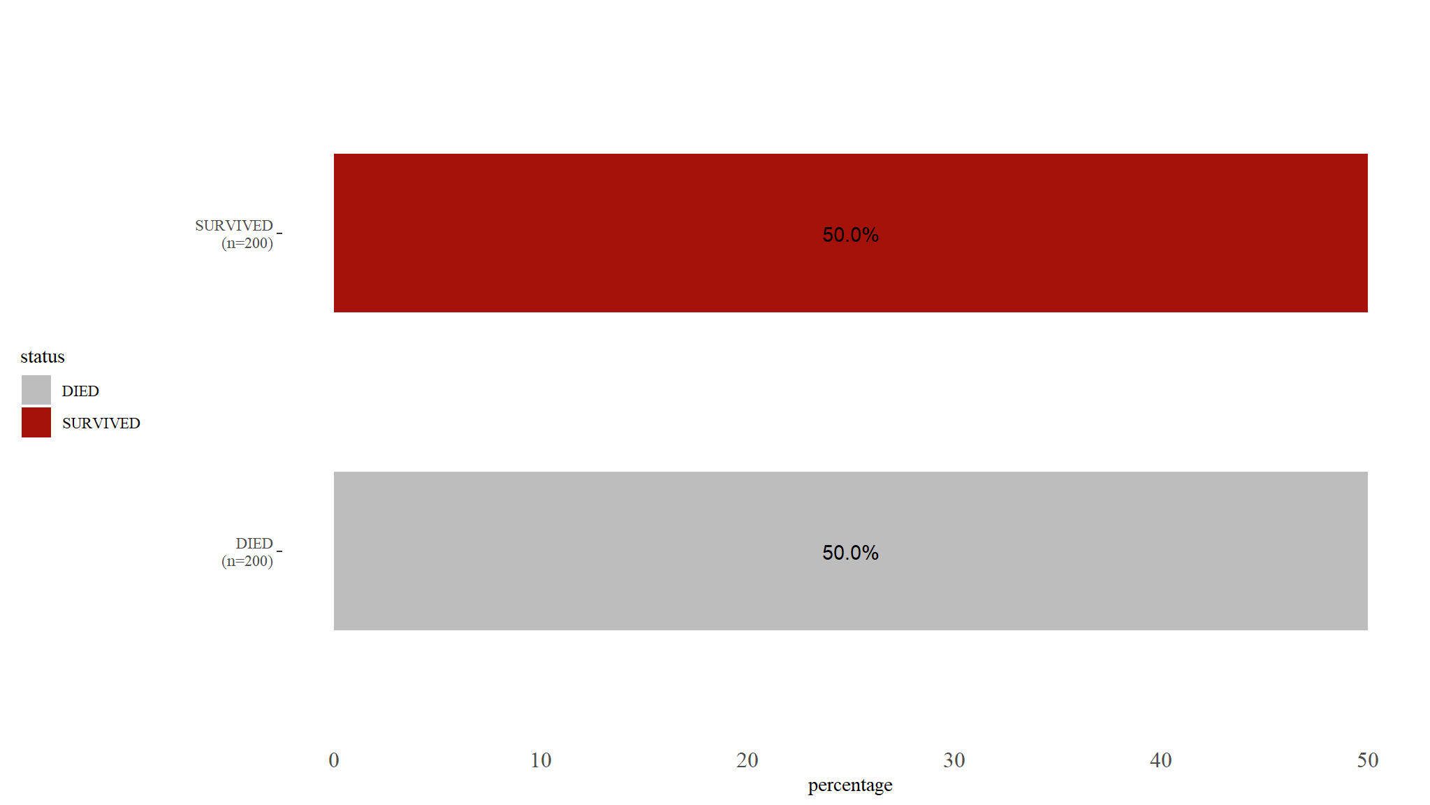
Comments
- lookas like our dataset was well balanced
Demographics
| Characteristic | DIED, N = 200 | SURVIVED, N = 200 | Test Statistic | p-value1 |
|---|---|---|---|---|
| husband_employed, n / N (%) | 0.66 | 0.42 | ||
| employed | 88 / 200 (44%) | 80 / 200 (40%) | ||
| Not employed | 112 / 200 (56%) | 120 / 200 (60%) | ||
| Birth tabattended, n / N (%) | 9.2 | 0.010 | ||
| Doctor | 37 / 200 (19%) | 49 / 200 (25%) | ||
| Nurse/Midwife | 158 / 200 (79%) | 135 / 200 (68%) | ||
| Traditional | 5 / 200 (2.5%) | 16 / 200 (8.0%) | ||
| Marital_Status, n / N (%) | 16 | 0.001 | ||
| Cohabiting | 104 / 200 (52%) | 108 / 200 (54%) | ||
| Married | 48 / 200 (24%) | 55 / 200 (28%) | ||
| other | 30 / 200 (15%) | 8 / 200 (4.0%) | ||
| Single | 18 / 200 (9.0%) | 29 / 200 (15%) | ||
| Reffered, n / N (%) | 2.6 | 0.11 | ||
| Not reffered | 156 / 200 (78%) | 142 / 200 (71%) | ||
| reffered | 44 / 200 (22%) | 58 / 200 (29%) | ||
| Education, n / N (%) | 74 | <0.001 | ||
| None | 52 / 200 (26%) | 55 / 200 (28%) | ||
| Primary | 61 / 200 (31%) | 86 / 200 (43%) | ||
| Secondary | 12 / 200 (6.0%) | 48 / 200 (24%) | ||
| Tertiary | 75 / 200 (38%) | 11 / 200 (5.5%) | ||
| Booking, n / N (%) | 107 | <0.001 | ||
| Booked | 79 / 200 (40%) | 178 / 200 (89%) | ||
| Not Booked | 121 / 200 (61%) | 22 / 200 (11%) | ||
| 1 Pearson’s Chi-squared test | ||||
Comments
- The table above presents the descriptive statistics of the variables of interest.
- It reveals that out of the 400 neonates sampled for the study, 200 of them survived and 200 died.
- The preliminary analysis using Pearson chi-square showed that booking status and Education level of the mother all had a \(p<0.001\) (\(<0.001\)) , Marital status of the mother and birth attendance also had significant \(p-value\) given by \(( \chi^2=16,p-value=0.001)\) and \(( \chi^2=9.2,p-value=0.01)\) respectively implying that the variables had significant association with the neonate’s status(died or survived).
- Employment status of the father and the variable reffered were seen not to be having significant association with the neonate’s status at \(5\%\) level of significance.
Clinical factors
| Characteristic | DIED, N = 200 | SURVIVED, N = 200 | Test Statistic | p-value1 |
|---|---|---|---|---|
| Mode, n / N (%) | 89 | <0.001 | ||
| C section | 62 / 200 (31%) | 110 / 200 (55%) | ||
| NVD | 59 / 200 (30%) | 87 / 200 (44%) | ||
| other | 79 / 200 (40%) | 3 / 200 (1.5%) | ||
| gestational_age, n / N (%) | 19 | <0.001 | ||
| above 32 | 43 / 200 (22%) | 83 / 200 (42%) | ||
| below 32 | 157 / 200 (79%) | 117 / 200 (59%) | ||
| COAF, n / N (%) | 14 | <0.001 | ||
| clear/yellow | 129 / 200 (65%) | 92 / 200 (46%) | ||
| green/brown | 71 / 200 (36%) | 108 / 200 (54%) | ||
| AMO, n / N (%) | 0.16 | 0.69 | ||
| foul | 114 / 200 (57%) | 118 / 200 (59%) | ||
| not foul | 86 / 200 (43%) | 82 / 200 (41%) | ||
| Parity, n / N (%) | 0.01 | 0.92 | ||
| adequate | 80 / 200 (40%) | 81 / 200 (41%) | ||
| High Risk | 120 / 200 (60%) | 119 / 200 (60%) | ||
| BirthWeight, n / N (%) | 112 | <0.001 | ||
| <1.5Kg | 117 / 200 (59%) | 17 / 200 (8.5%) | ||
| 1.5-2.5Kg | 83 / 200 (42%) | 183 / 200 (92%) | ||
| Maternal age, n / N (%) | 21 | <0.001 | ||
| 15-25 | 31 / 191 (16%) | 46 / 199 (23%) | ||
| 25-29 | 32 / 191 (17%) | 61 / 199 (31%) | ||
| 30-39 | 81 / 191 (42%) | 47 / 199 (24%) | ||
| 40+ | 47 / 191 (25%) | 45 / 199 (23%) | ||
| Unknown | 9 | 1 | ||
| preterm_rapture, n / N (%) | 18 | <0.001 | ||
| no | 43 / 200 (22%) | 82 / 200 (41%) | ||
| yes | 157 / 200 (79%) | 118 / 200 (59%) | ||
| 1 Pearson’s Chi-squared test | ||||
Comments
- Table above shows the frequency and tests for independence between the categorical variable that are more clinical and the outcome variable of a neonate, the first variable is mode and has three categories which are C section, NVD and other.
- The test statistic is 89, with a very small \(p-value\) indicating a strong association between the mode of delivery and the outcome variable.
- Another variable is gestational age and has two categories: above 32 weeks and below 32 weeks ,the results from the chi-squared test indicate that that there is strong association between gestational age and the outcome variable \((\chi^2=19,p<10001)\).
- fluid odour on the other hand has two categories: foul and not foul. The test statistic is \(\chi^2= 0.16)\), with a p-value of 0.69, indicating no significant association between fluid odour and the outcome death of the neonates .
- Another variable is parity and has two categories: adequate and high risk, the result show \((\chi^2=0.01, p-value= 0.92)\), indicating no significant association between parity and the outcome event of the neonate.
- Birth weight was also considered and has two categories: less than 1.5 Kg and 1.5-2.5 Kg, table shows that \((\chi^2=112, p-value<0.001)\), indicating a significant association between birth weight and the final event outcome of a neonate.
- The seventh characteristic, maternal age, has four categories: \(15-25\), \(25-29\), \(30-39\), and \(40+\).
- The test statistic is 21, with a very small p-value, indicating a significant association between maternal age and the outcome and the outcome of death.
- Preterm rupture, has two categories: yes and no,the test statistic of 18, has a corresponding \(p-value\) \((p<0001)\) indicating a significant association between preterm rupture and death of a neonate.
further exploration on
- Out of interest , research shows that babies born preterm have a higher risk of dying
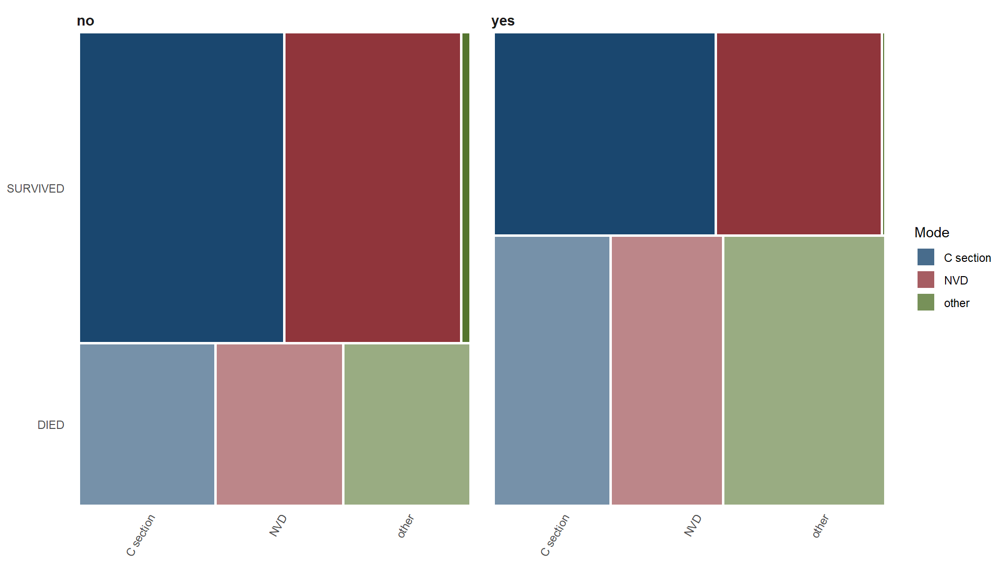
Whats the relationship between death, preterm rapture and mode of delivery
| C section | NVD | other | |
|---|---|---|---|
| DIED | |||
| no | 34.88% |
32.56% |
32.56% |
| yes | 29.94% |
28.66% |
41.40% |
| SURVIVED | |||
| no | 52.44% |
45.12% |
2.44% |
| yes | 56.78% |
42.37% |
0.85% |
C section vs DIED==Yes
| C section | NVD | other | |
|---|---|---|---|
| DIED | |||
| no | 34.88% |
32.56% |
32.56% |
| yes | 29.94% |
28.66% |
41.40% |
| SURVIVED | |||
| no | 52.44% |
45.12% |
2.44% |
| yes | 56.78% |
42.37% |
0.85% |
Proportions
#>      n_often n_not_often
#> [1,]      15          28
#> [2,]      47         110
Proportional test for those who died and had C section
#> 2-sample test for equality of proportions
#>
#> Proportion      | Difference |        95% CI | Chi2(1) |     p
#> --------------------------------------------------------------
#> 34.88% / 29.94% |      4.95% | [-0.12, 0.22] |    0.19 | 0.663
#>
#> Alternative hypothesis: two.sided
Comments
- for our study ,we found a value of 0.19, which is small and definitely statistically insignificant. In a hypothetical world where there’s no difference in the proportions, the probability of seeing a difference of at least \(4.95\) percentage points is super huge (p = 0.663).
- We have enough evidence to confidently accept the null hypothesis and declare that the proportions of the groups are are the same. With the confidence interval, we can say that we are 95% confident that the interval [-0.12, 0.22] captures the true population parameter.
- however We can’t say that there’s a 95% chance that the true value falls in this range—we can only talk about the range.
Survival Analysis
Instantaneous Hazard
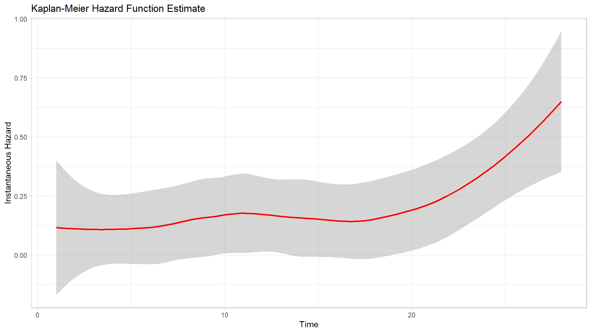
Comments
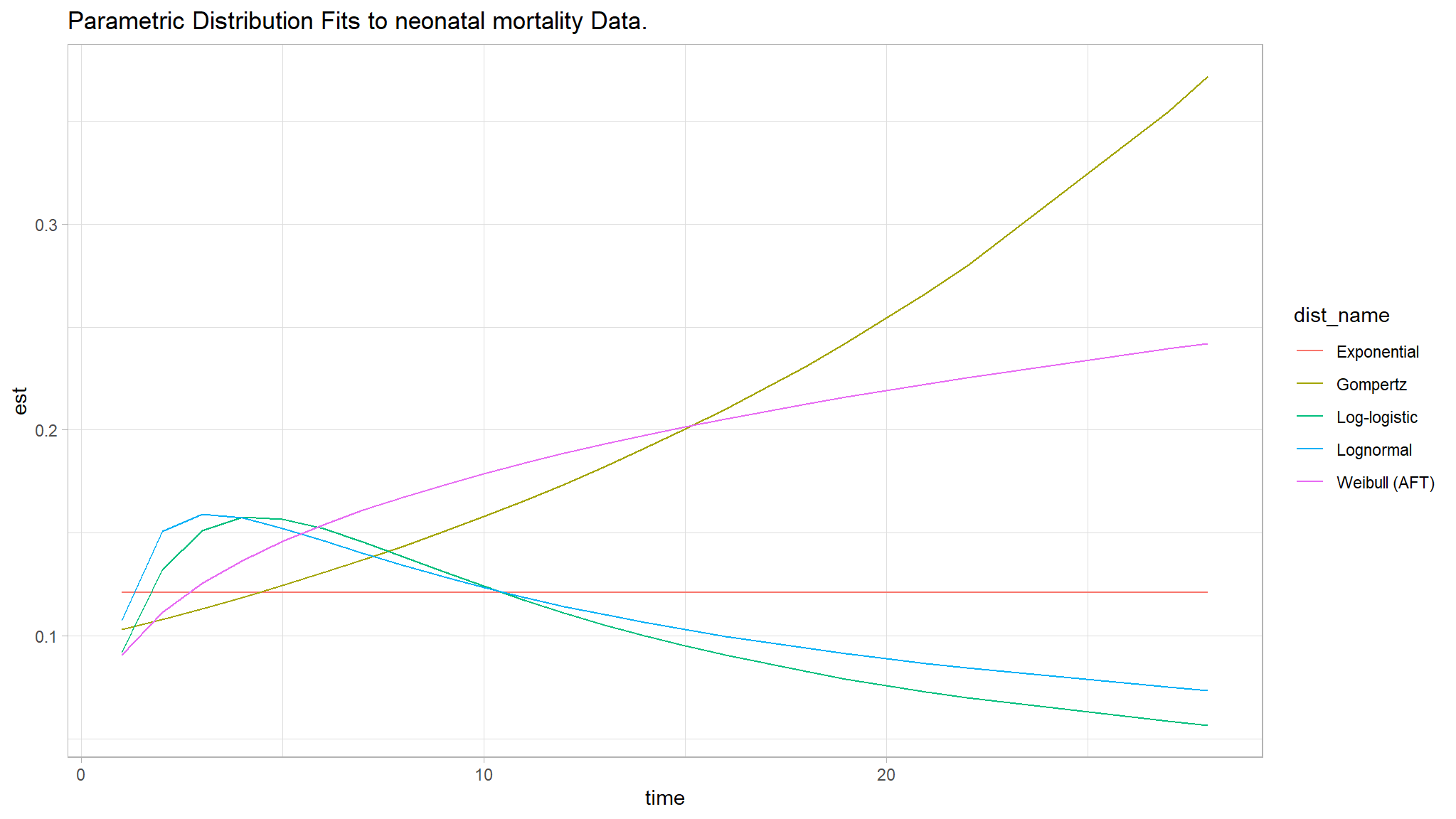
- The Figure above is found after fitting null models for exponential, Cox PH, log-logistic, lognormal, weibull (PH) and weibull (AFT), none of them seemed great.
- The three curves Weibull (AFT), Log-logistic and Log-normal seem especially better choices.
- We further analyzed goodness of fit for the null models using the Akaike Information criterion .
Comments
Using the AIC, the best fit model appears to be the lognormal model since it has the least AIC value of \(1222.156\) as compared to other models.
Thus the prelimenary analysis of the null models show that the Lognormal AFT and the Weibull (PH) seem to be better fit for the null models.
kaplan Meier Curves
Comments
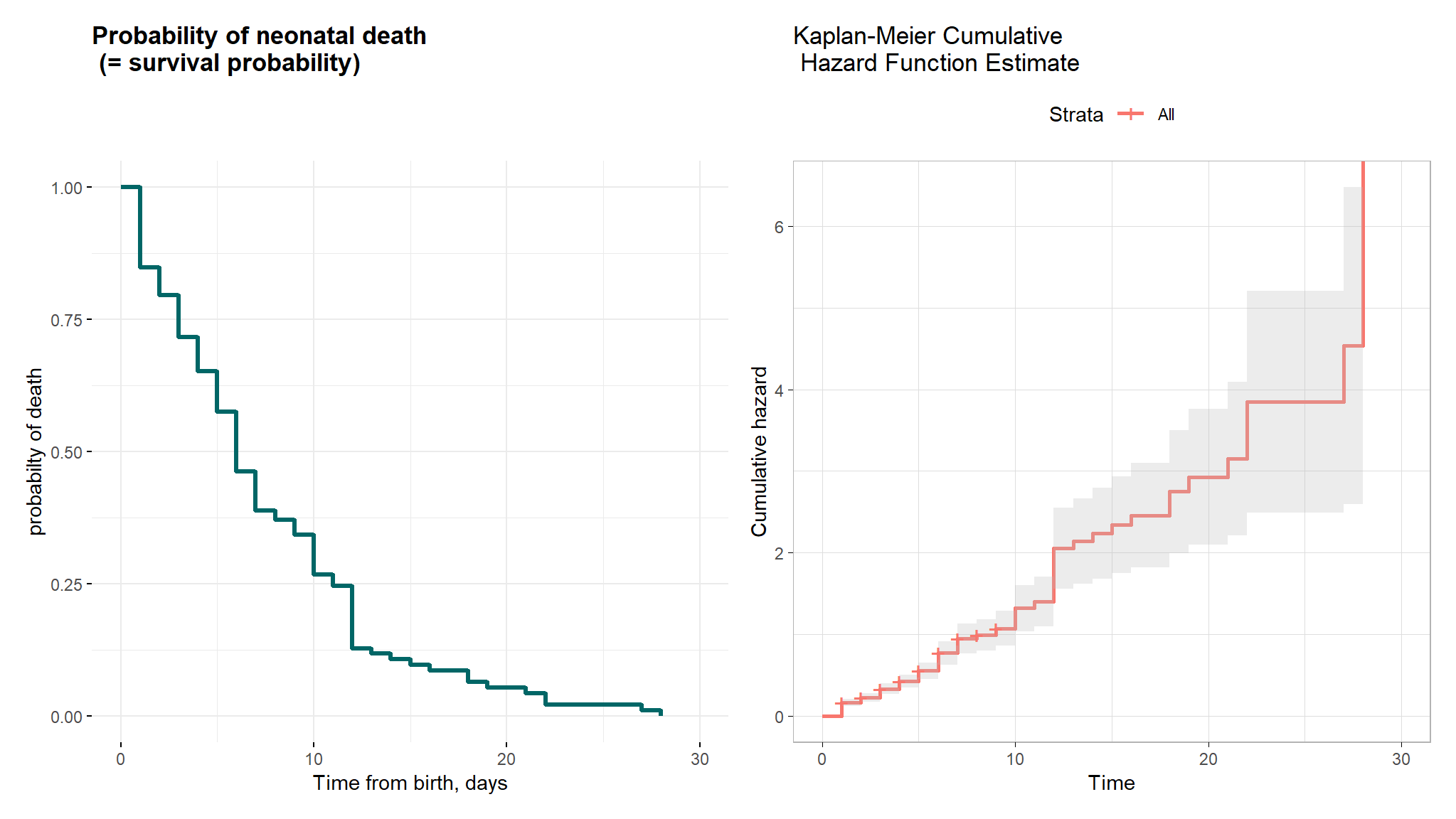
- The mean and median overall survival times for neonates were 4.135 and 3 days, respectively.
- The minimum and maximum survival times observed were 1 and 28 days, respectively.
- These findings suggest that neonates, on average, experience death after 4 days from birth, with some neonates dying as early as the first day and as late as the 28th day.
- the Kaplan-Meier curve showing the probability of neonatal survival and shows the actual survival times and the probability of survival over time.
- The Kaplan-Meier cumulative hazard function estimate revealed that the cumulative hazard rises more sharply at around times 12, 23, and 27 days. This information provides insight into the timing and frequency of events and can help to identify potential risk factors for neonatal mortality.
Gender and Color of Amniotic fluid
Comments
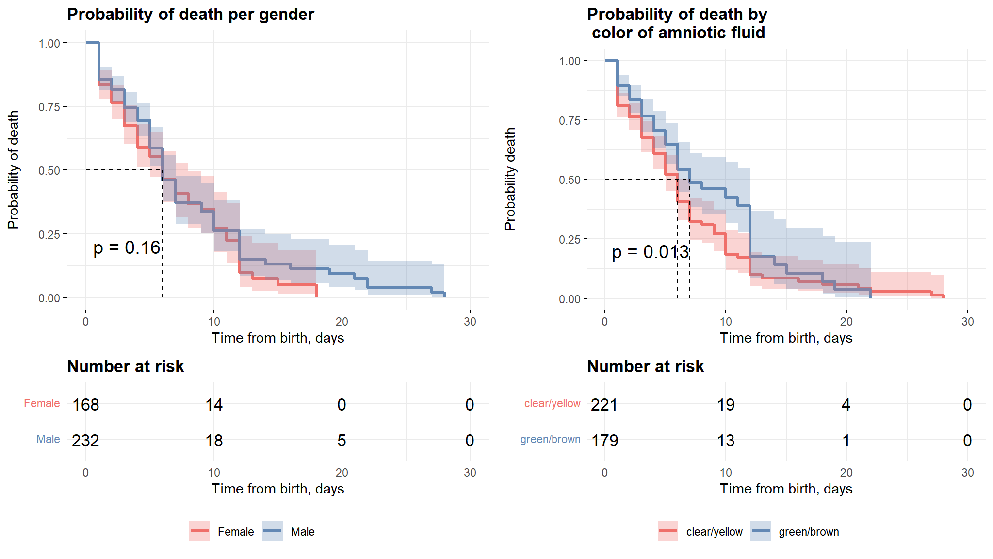
The plots above show the difference in survival times for the selected variables. it can be noticed that there is no significant difference in survival times between males and females, this result is also further clarified by the logrank test which will proceed in the coming sections.
The second plot shows that neonates with clear/yellow fluid color have more survival time as compared to the other group and this can also be explained by the log rank test.
kaplan meier estimates gestational age And amniotic fluid odour
Comments
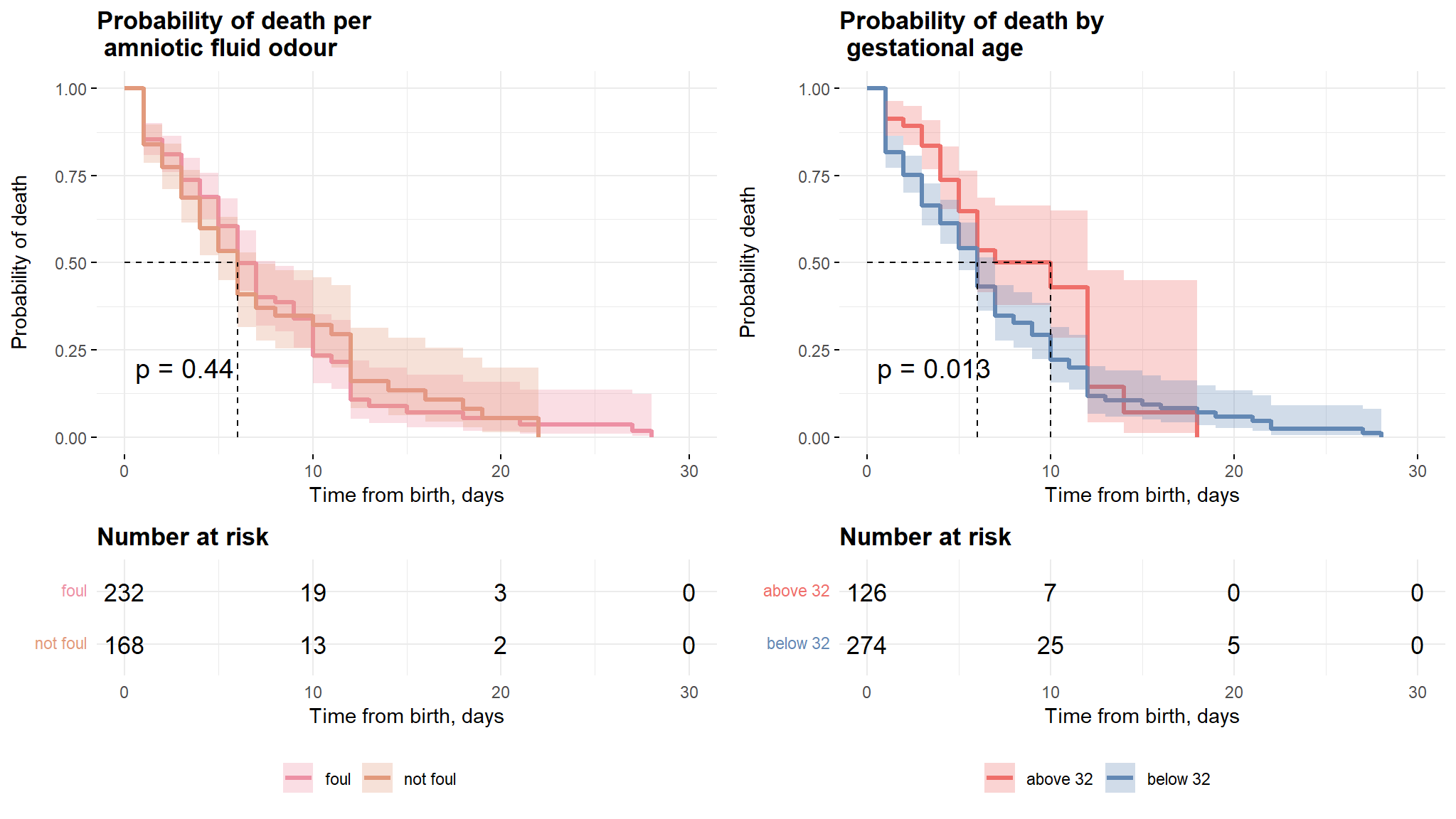
- The first plot from figure above shows that there is no significant difference in survival times of neonates with foul and non foul amniotic fluid.
- The second plot however reveals that the neonates with gestational age above 32 weeks have a longer survival time as compared to their counterparts with age less that 32 weeks.
Mode of delivery and Birthweight
Comments
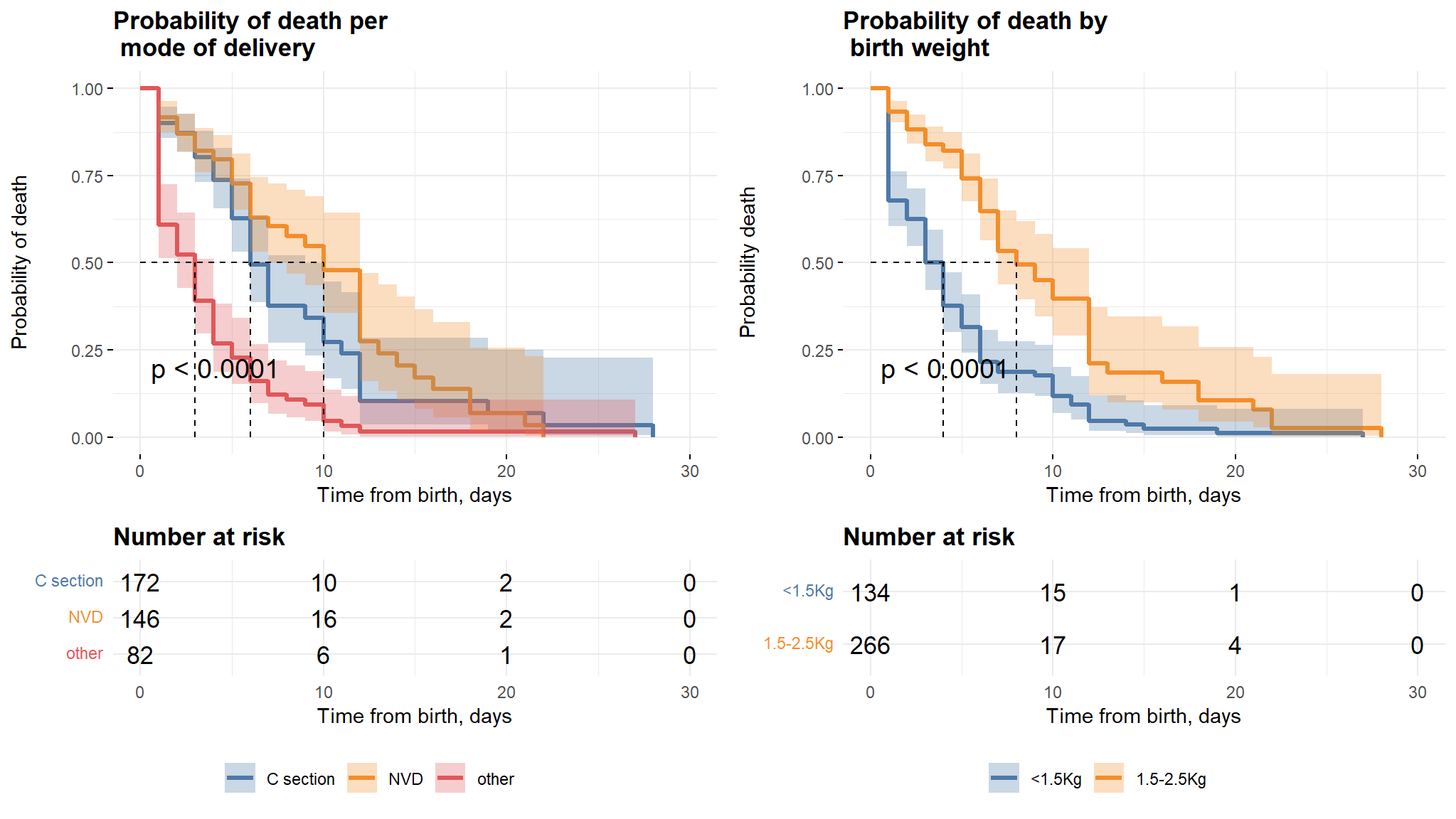
- It can be noted from the first plot that, babies whose mothers have a Normal Vaginal Delivery (NVD) survived longer as compared to those who had Caesarian section and other modes.
- Babies born with weight between 1.5-2.5kg also survived longer than those with weight below 1.5 kg.
Preterm Rapture And Parity
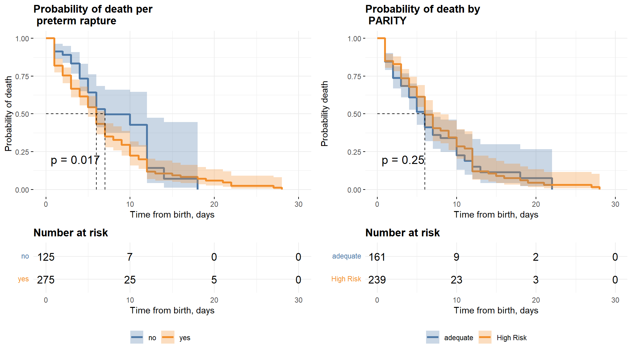
Comments
- It can be noted from the first graph that neonates whose mothers did not have a preterm rapture have a longer survival time as compared to those whose mothers had a preterm rapture.
- There is however no difference in survival times for the two classes in the parity variable.
Univariate Cox and Univariate Logistic regression
| Characteristic | Death Status | Time to Death | ||||
|---|---|---|---|---|---|---|
| N | OR (95% CI)1 | p-value | N | HR (95% CI)1 | p-value | |
| Birth_attended | 400 | 400 | ||||
| Doctor | — | — | ||||
| Nurse/Midwife | 1.55 (0.96 to 2.53) | 0.076 | 1.12 (0.78 to 1.60) | 0.54 | ||
| Traditional | 0.41 (0.13 to 1.16) | 0.11 | 0.69 (0.27 to 1.77) | 0.44 | ||
| Parity | 400 | 400 | ||||
| adequate | — | — | ||||
| High Risk | 1.02 (0.68 to 1.52) | 0.92 | 0.85 (0.64 to 1.14) | 0.28 | ||
| gender | 400 | 400 | ||||
| Female | — | — | ||||
| Male | 0.88 (0.59 to 1.32) | 0.54 | 0.82 (0.62 to 1.09) | 0.18 | ||
| BirthWeight | 400 | 400 | ||||
| <1.5Kg | — | — | ||||
| 1.5-2.5Kg | 0.07 (0.04 to 0.11) | <0.001 | 0.33 (0.25 to 0.44) | <0.001 | ||
| COAF | 400 | 400 | ||||
| clear/yellow | — | — | ||||
| green/brown | 0.47 (0.31 to 0.70) | <0.001 | 0.70 (0.52 to 0.93) | 0.015 | ||
| AMO | 400 | 400 | ||||
| foul | — | — | ||||
| not foul | 1.09 (0.73 to 1.62) | 0.69 | 1.11 (0.84 to 1.47) | 0.46 | ||
| Mode | 400 | 400 | ||||
| C section | — | — | ||||
| NVD | 1.20 (0.76 to 1.90) | 0.42 | 0.75 (0.52 to 1.08) | 0.12 | ||
| other | 46.7 (16.6 to 196) | <0.001 | 2.90 (2.08 to 4.06) | <0.001 | ||
| Maternal_age | 390 | 390 | ||||
| 15-25 | — | — | ||||
| 25-29 | 0.78 (0.42 to 1.46) | 0.43 | 0.83 (0.50 to 1.36) | 0.45 | ||
| 30-39 | 2.56 (1.44 to 4.60) | 0.002 | 1.21 (0.80 to 1.84) | 0.37 | ||
| 40+ | 1.55 (0.84 to 2.87) | 0.16 | 1.12 (0.71 to 1.76) | 0.64 | ||
| gestational_age | 400 | 400 | ||||
| above 32 | — | — | ||||
| below 32 | 2.59 (1.68 to 4.04) | <0.001 | 1.51 (1.08 to 2.13) | 0.017 | ||
| preterm_rapture | 400 | 400 | ||||
| no | — | — | ||||
| yes | 2.54 (1.64 to 3.96) | <0.001 | 1.49 (1.06 to 2.10) | 0.021 | ||
| HIE | 400 | 400 | ||||
| no | — | — | ||||
| yes | 41.4 (12.7 to 255) | <0.001 | 15.3 (3.80 to 61.8) | <0.001 | ||
| 1 OR = Odds Ratio, CI = Confidence Interval, HR = Hazard Ratio, CI = Confidence Interval | ||||||
Comments
- the table above shows individual univariate Cox and logistic regression models
- the univariate models help to add more details to the chi-square tests as with the chisquare tests we note the following :
Multivariate Cox and Logistic Regression
| Characteristic | Logistic | Cox PH | ||
|---|---|---|---|---|
| HR (95% CI)1 | p-value | OR (95% CI)1 | p-value | |
| Birth_attended | ||||
| Doctor | — | — | ||
| Nurse/Midwife | 1.23 (0.82 to 1.82) | 0.31 | 1.57 (0.79 to 3.17) | 0.20 |
| Traditional | 1.14 (0.43 to 3.00) | 0.79 | 0.30 (0.05 to 1.36) | 0.15 |
| Parity | ||||
| adequate | — | — | ||
| High Risk | 0.88 (0.64 to 1.22) | 0.46 | 1.28 (0.68 to 2.44) | 0.45 |
| gender | ||||
| Female | — | — | ||
| Male | 1.06 (0.78 to 1.45) | 0.71 | 1.82 (1.02 to 3.33) | 0.046 |
| BirthWeight | ||||
| <1.5Kg | — | — | ||
| 1.5-2.5Kg | 0.46 (0.31 to 0.67) | <0.001 | 0.10 (0.04 to 0.23) | <0.001 |
| COAF | ||||
| clear/yellow | — | — | ||
| green/brown | 0.77 (0.55 to 1.09) | 0.14 | 0.58 (0.32 to 1.06) | 0.077 |
| AMO | ||||
| foul | — | — | ||
| not foul | 1.40 (1.00 to 1.96) | 0.047 | 1.40 (0.78 to 2.55) | 0.26 |
| Mode | ||||
| C section | — | — | ||
| NVD | 0.72 (0.49 to 1.07) | 0.10 | 1.09 (0.60 to 1.98) | 0.78 |
| other | 1.59 (1.05 to 2.40) | 0.028 | 18.6 (4.47 to 134) | <0.001 |
| Maternal_age | ||||
| 15-25 | — | — | ||
| 25-29 | 0.79 (0.48 to 1.31) | 0.36 | 0.75 (0.31 to 1.81) | 0.53 |
| 30-39 | 0.85 (0.54 to 1.33) | 0.48 | 2.38 (1.02 to 5.68) | 0.048 |
| 40+ | 0.83 (0.51 to 1.37) | 0.47 | 2.01 (0.83 to 4.93) | 0.12 |
| gestational_age | ||||
| above 32 | — | — | ||
| below 32 | 1.31 (0.92 to 1.87) | 0.14 | 3.05 (1.62 to 5.96) | <0.001 |
| HIE | ||||
| no | — | — | ||
| yes | 9.54 (2.34 to 38.8) | 0.002 | 111 (18.8 to 1,397) | <0.001 |
| 1 HR = Hazard Ratio, CI = Confidence Interval, OR = Odds Ratio, CI = Confidence Interval | ||||
Model diagnostics for Cox Regression
Deviance Residuals
Dfbeta
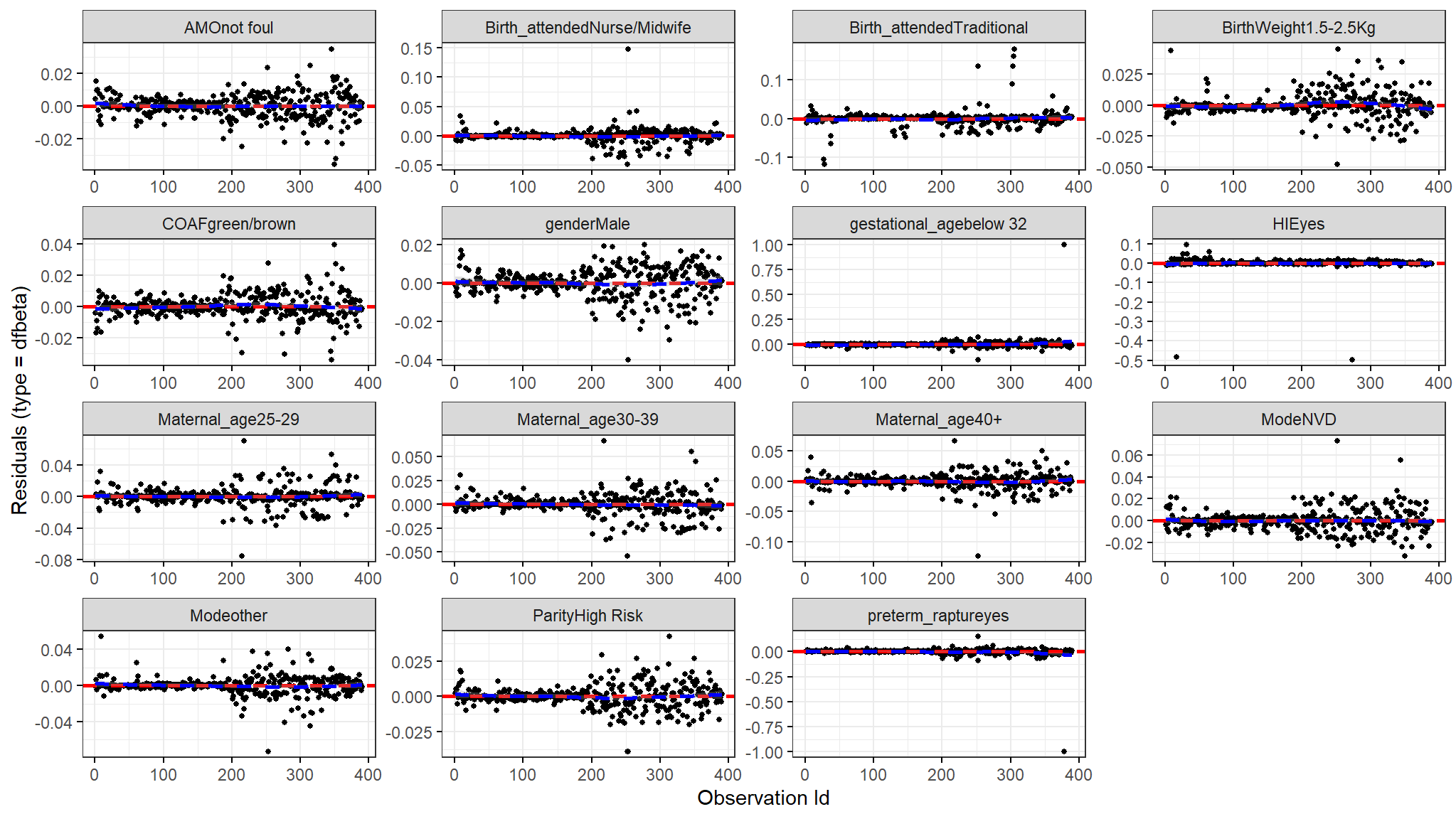
Comments
- The figure above shows the estimated changes that are found in the regression coefficients that are observed from removing each observation one after the other.
- We compare size in values of the largest dfbetas values to the regression coefficients and as seen from the plot above none of the observations is very influential.
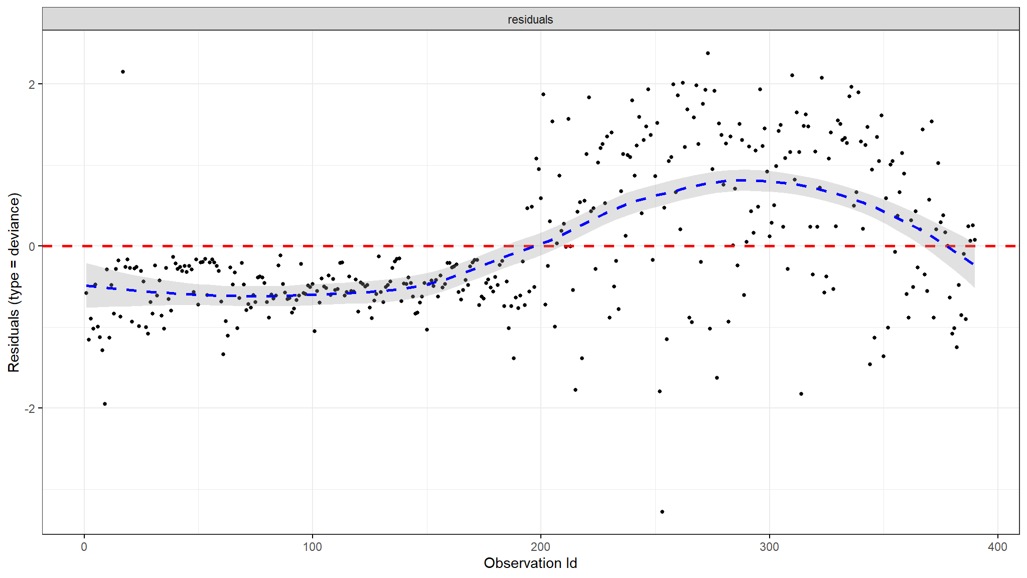
Martingale and Deviance Residuals
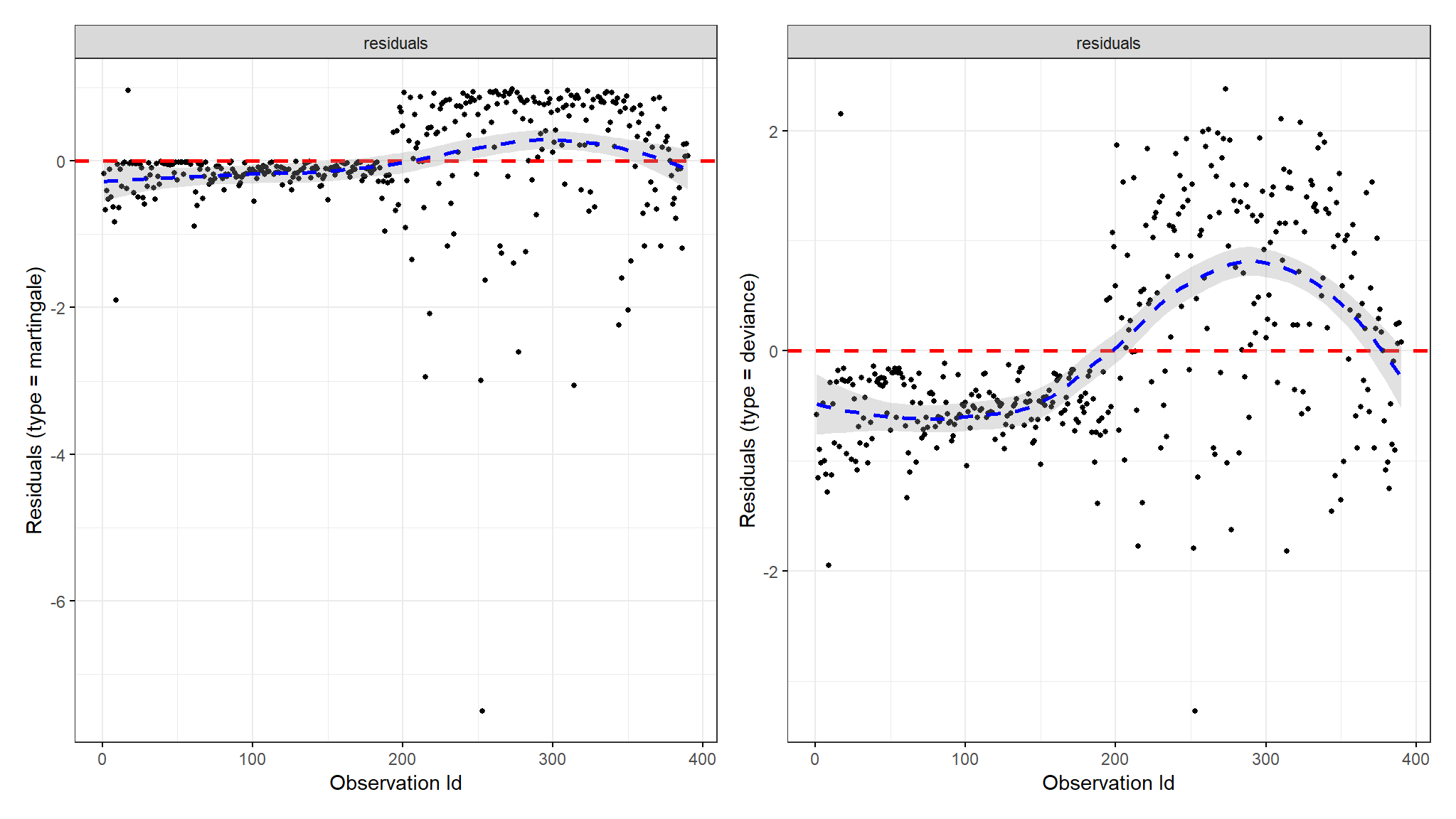
Comments
- one of the plots shows deviance residuals which are normalized transformations of the Martingale residuals.
- Deviance residuals should be symmetrically distributed about zero as shown in the plot with a standard deviation of 1 for the proportional hazard assumption to hold.
Parametric models
Univariate Weibull model
| Characteristic | N | exp(Beta) (95% CI)1 | p-value |
|---|---|---|---|
| Birth_attended | 400 | ||
| Doctor | — | ||
| Nurse/Midwife | -0.07 (-0.35 to 0.21) | 0.63 | |
| Traditional | 0.23 (-0.49 to 0.96) | 0.53 | |
| Parity | 400 | ||
| adequate | — | ||
| High Risk | 0.14 (-0.08 to 0.35) | 0.22 | |
| gender | 400 | ||
| Female | — | ||
| Male | 0.17 (-0.05 to 0.38) | 0.13 | |
| BirthWeight | 400 | ||
| <1.5Kg | — | ||
| 1.5-2.5Kg | 0.79 (0.56 to 1.02) | <0.001 | |
| COAF | 400 | ||
| clear/yellow | — | ||
| green/brown | 0.25 (0.02 to 0.47) | 0.034 | |
| AMO | 400 | ||
| foul | — | ||
| not foul | -0.09 (-0.30 to 0.13) | 0.44 | |
| Mode | 400 | ||
| C section | — | ||
| NVD | 0.27 (0.00 to 0.55) | 0.049 | |
| other | -0.70 (-0.96 to -0.44) | <0.001 | |
| Maternal_age | 390 | ||
| 15-25 | — | ||
| 25-29 | 0.17 (-0.22 to 0.55) | 0.39 | |
| 30-39 | -0.09 (-0.42 to 0.23) | 0.57 | |
| 40+ | -0.04 (-0.40 to 0.31) | 0.81 | |
| gestational_age | 400 | ||
| above 32 | — | ||
| below 32 | -0.29 (-0.56 to -0.02) | 0.036 | |
| preterm_rapture | 400 | ||
| no | — | ||
| yes | -0.28 (-0.55 to -0.01) | 0.043 | |
| HIE | 400 | ||
| no | — | ||
| yes | -2.12 (-3.27 to -0.97) | <0.001 | |
| 1 CI = Confidence Interval | |||
Multivariate Weibul PH model
| Weibull model | |||
| Independent Variables | N | exp(Beta) (95% CI)1 | p-value |
|---|---|---|---|
| (Intercept) | 390 | 3.45 (2.19 to 4.70) | <0.001 |
| Birth_attended | 390 | ||
| Doctor | — | ||
| Nurse/Midwife | -0.15 (-0.46 to 0.15) | 0.33 | |
| Traditional | -0.21 (-0.95 to 0.54) | 0.59 | |
| Parity | 390 | ||
| adequate | — | ||
| High Risk | 0.11 (-0.14 to 0.36) | 0.39 | |
| gender | 390 | ||
| Female | — | ||
| Male | -0.03 (-0.28 to 0.21) | 0.78 | |
| BirthWeight | 390 | ||
| <1.5Kg | — | ||
| 1.5-2.5Kg | 0.56 (0.26 to 0.85) | <0.001 | |
| COAF | 390 | ||
| clear/yellow | — | ||
| green/brown | 0.17 (-0.10 to 0.44) | 0.21 | |
| AMO | 390 | ||
| foul | — | ||
| not foul | -0.26 (-0.52 to 0.00) | 0.054 | |
| Mode | 390 | ||
| C section | — | ||
| NVD | 0.30 (0.01 to 0.60) | 0.045 | |
| other | -0.30 (-0.62 to 0.02) | 0.064 | |
| Maternal_age | 390 | ||
| 15-25 | — | ||
| 25-29 | 0.21 (-0.18 to 0.60) | 0.29 | |
| 30-39 | 0.16 (-0.18 to 0.50) | 0.36 | |
| 40+ | 0.21 (-0.16 to 0.59) | 0.27 | |
| gestational_age | 390 | ||
| above 32 | — | ||
| below 32 | -11.8 (-5,298 to 5,274) | >0.99 | |
| preterm_rapture | 390 | ||
| no | — | ||
| yes | 11.7 (-5,274 to 5,297) | >0.99 | |
| HIE | 390 | ||
| no | — | ||
| yes | -1.70 (-2.80 to -0.60) | 0.002 | |
| iter = 15.0; df = 17; Statistic = 108; Log-likelihood = -532; AIC = 1,098; BIC = 1,165; Residual df = 373; No. Obs. = 390; p-value = <0.001 | |||
| 1 CI = Confidence Interval | |||
Multivariate lognormal PH model
| Lognormal model | |||
| Independent Variables | N | exp(Beta) (95% CI)1 | p-value |
|---|---|---|---|
| (Intercept) | 390 | 2.52 (1.68 to 3.37) | <0.001 |
| Birth_attended | 390 | ||
| Doctor | — | ||
| Nurse/Midwife | -0.01 (-0.30 to 0.28) | 0.94 | |
| Traditional | 0.09 (-0.57 to 0.75) | 0.79 | |
| Parity | 390 | ||
| adequate | — | ||
| High Risk | 0.15 (-0.10 to 0.40) | 0.25 | |
| gender | 390 | ||
| Female | — | ||
| Male | -0.08 (-0.32 to 0.16) | 0.51 | |
| BirthWeight | 390 | ||
| <1.5Kg | — | ||
| 1.5-2.5Kg | 0.57 (0.29 to 0.86) | <0.001 | |
| COAF | 390 | ||
| clear/yellow | — | ||
| green/brown | 0.18 (-0.09 to 0.45) | 0.19 | |
| AMO | 390 | ||
| foul | — | ||
| not foul | -0.25 (-0.51 to 0.02) | 0.069 | |
| Mode | 390 | ||
| C section | — | ||
| NVD | 0.31 (0.03 to 0.59) | 0.032 | |
| other | -0.37 (-0.70 to -0.04) | 0.030 | |
| Maternal_age | 390 | ||
| 15-25 | — | ||
| 25-29 | 0.25 (-0.13 to 0.63) | 0.20 | |
| 30-39 | 0.14 (-0.20 to 0.49) | 0.41 | |
| 40+ | 0.18 (-0.19 to 0.56) | 0.34 | |
| gestational_age | 390 | ||
| above 32 | — | ||
| below 32 | -4.53 (-1,148 to 1,138) | >0.99 | |
| preterm_rapture | 390 | ||
| no | — | ||
| yes | 4.24 (-1,139 to 1,147) | >0.99 | |
| HIE | 390 | ||
| no | — | ||
| yes | -1.24 (-1.87 to -0.60) | <0.001 | |
| iter = 12.0; df = 17; Statistic = 125; Log-likelihood = -521; AIC = 1,077; BIC = 1,144; Residual df = 373; No. Obs. = 390; p-value = <0.001 | |||
| 1 CI = Confidence Interval | |||
Multivariate exponential PH model
| exponential model | |||
| Independent Variables | N | exp(Beta) (95% CI)1 | p-value |
|---|---|---|---|
| (Intercept) | 390 | 4.19 (2.60 to 5.78) | <0.001 |
| Birth_attended | 390 | ||
| Doctor | — | ||
| Nurse/Midwife | -0.17 (-0.56 to 0.22) | 0.40 | |
| Traditional | -0.02 (-0.98 to 0.94) | 0.97 | |
| Parity | 390 | ||
| adequate | — | ||
| High Risk | 0.09 (-0.23 to 0.42) | 0.56 | |
| gender | 390 | ||
| Female | — | ||
| Male | -0.07 (-0.38 to 0.23) | 0.64 | |
| BirthWeight | 390 | ||
| <1.5Kg | — | ||
| 1.5-2.5Kg | 0.69 (0.32 to 1.06) | <0.001 | |
| COAF | 390 | ||
| clear/yellow | — | ||
| green/brown | 0.22 (-0.12 to 0.56) | 0.21 | |
| AMO | 390 | ||
| foul | — | ||
| not foul | -0.29 (-0.62 to 0.04) | 0.085 | |
| Mode | 390 | ||
| C section | — | ||
| NVD | 0.31 (-0.07 to 0.69) | 0.11 | |
| other | -0.38 (-0.79 to 0.02) | 0.065 | |
| Maternal_age | 390 | ||
| 15-25 | — | ||
| 25-29 | 0.22 (-0.28 to 0.72) | 0.39 | |
| 30-39 | 0.10 (-0.34 to 0.55) | 0.64 | |
| 40+ | 0.16 (-0.33 to 0.64) | 0.53 | |
| gestational_age | 390 | ||
| above 32 | — | ||
| below 32 | -15.2 (-5,858 to 5,827) | >0.99 | |
| preterm_rapture | 390 | ||
| no | — | ||
| yes | 15.0 (-5,828 to 5,858) | >0.99 | |
| HIE | 390 | ||
| no | — | ||
| yes | -2.33 (-3.73 to -0.93) | 0.001 | |
| iter = 15.0; df = 16; Statistic = 109; Log-likelihood = -543; AIC = 1,118; BIC = 1,181; Residual df = 374; No. Obs. = 390; p-value = <0.001 | |||
| 1 CI = Confidence Interval | |||
Multivariate loglogistic PH model
| loglogistic model | |||
| Independent Variables | N | exp(Beta) (95% CI)1 | p-value |
|---|---|---|---|
| (Intercept) | 390 | 2.61 (1.63 to 3.58) | <0.001 |
| Birth_attended | 390 | ||
| Doctor | — | ||
| Nurse/Midwife | 0.02 (-0.29 to 0.33) | 0.90 | |
| Traditional | 0.05 (-0.61 to 0.71) | 0.89 | |
| Parity | 390 | ||
| adequate | — | ||
| High Risk | 0.19 (-0.07 to 0.45) | 0.16 | |
| gender | 390 | ||
| Female | — | ||
| Male | -0.12 (-0.37 to 0.13) | 0.34 | |
| BirthWeight | 390 | ||
| <1.5Kg | — | ||
| 1.5-2.5Kg | 0.58 (0.28 to 0.89) | <0.001 | |
| COAF | 390 | ||
| clear/yellow | — | ||
| green/brown | 0.19 (-0.09 to 0.46) | 0.19 | |
| AMO | 390 | ||
| foul | — | ||
| not foul | -0.25 (-0.52 to 0.02) | 0.067 | |
| Mode | 390 | ||
| C section | — | ||
| NVD | 0.29 (-0.01 to 0.59) | 0.057 | |
| other | -0.45 (-0.80 to -0.11) | 0.010 | |
| Maternal_age | 390 | ||
| 15-25 | — | ||
| 25-29 | 0.24 (-0.15 to 0.64) | 0.23 | |
| 30-39 | 0.19 (-0.16 to 0.55) | 0.29 | |
| 40+ | 0.19 (-0.19 to 0.58) | 0.32 | |
| gestational_age | 390 | ||
| above 32 | — | ||
| below 32 | -8.50 (-3,920 to 3,903) | >0.99 | |
| preterm_rapture | 390 | ||
| no | — | ||
| yes | 8.22 (-3,903 to 3,920) | >0.99 | |
| HIE | 390 | ||
| no | — | ||
| yes | -1.33 (-2.13 to -0.53) | 0.001 | |
| iter = 14.0; df = 17; Statistic = 127; Log-likelihood = -527; AIC = 1,088; BIC = 1,155; Residual df = 373; No. Obs. = 390; p-value = <0.001 | |||
| 1 CI = Confidence Interval | |||
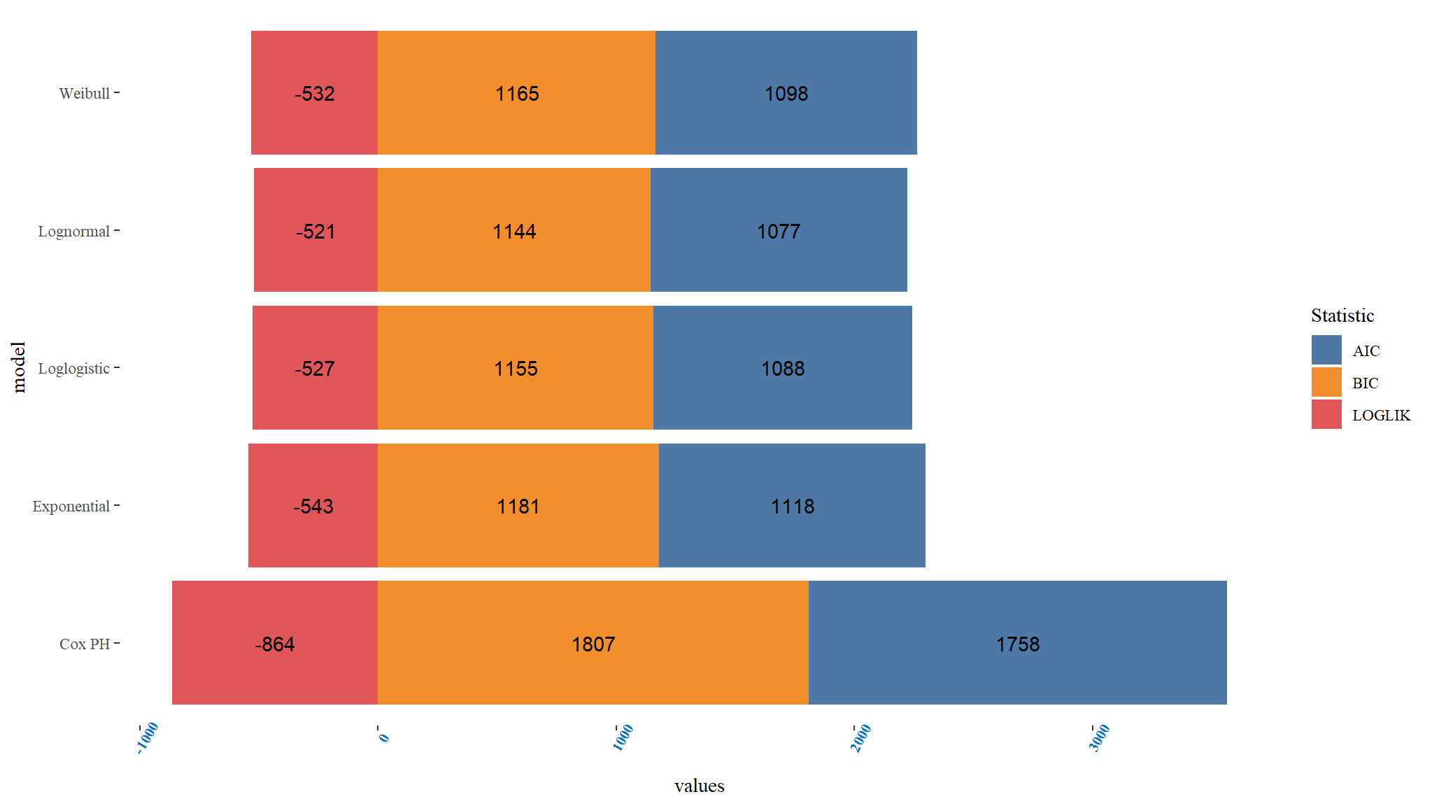
Comparing PH models
Comments
- it can be noted that the Lognormal PH model has the least
Bayesian information and Akaike information Criterionhence can be chosen as the best model among the PH Models. - The loglikelihood also further confirms that the Lognormal is the best fitting model since it is smallest for the Lognormal model.
- Overally it means that the Lognormal model is the best fitting among the parametric hazard models for the given dataset.
Accelerated failure time MODELS
Weibull AFT
#> Call:
#> aftreg(formula = Surv(days, DEATH) ~ Birth_attended + Parity +
#>     gender + BirthWeight + COAF + AMO + Birth_attended + Mode +
#>     Maternal_age + gestational_age + preterm_rapture + HIE, data = out_new,
#>     dist = "weibull")
#>
#> Covariate          W.mean      Coef Time-Accn  se(Coef)    Wald p
#> Birth_attended
#>           Doctor    0.207     0         1           (reference)
#>    Nurse/Midwife    0.751     0.153     1.166     0.156     0.326
#>      Traditional    0.042     0.207     1.230     0.380     0.586
#> Parity
#>         adequate    0.378     0         1           (reference)
#>        High Risk    0.622    -0.110     0.896     0.127     0.387
#> gender
#>           Female    0.387     0         1           (reference)
#>             Male    0.613     0.035     1.035     0.123     0.779
#> BirthWeight
#>           <1.5Kg    0.331     0         1           (reference)
#>        1.5-2.5Kg    0.669    -0.555     0.574     0.149     0.000
#> COAF
#>     clear/yellow    0.572     0         1           (reference)
#>      green/brown    0.428    -0.171     0.843     0.136     0.209
#> AMO
#>             foul    0.601     0         1           (reference)
#>         not foul    0.399     0.256     1.291     0.133     0.054
#> Mode
#>        C section    0.344     0         1           (reference)
#>              NVD    0.473    -0.301     0.740     0.150     0.045
#>            other    0.184     0.299     1.349     0.161     0.063
#> Maternal_age
#>            15-25    0.172     0         1           (reference)
#>            25-29    0.221    -0.209     0.811     0.198     0.290
#>            30-39    0.370    -0.161     0.851     0.175     0.355
#>              40+    0.237    -0.214     0.807     0.192     0.265
#> gestational_age
#>         above 32    0.301     0         1           (reference)
#>         below 32    0.699     6.446   630.254    80.932     0.937
#> preterm_rapture
#>               no    0.298     0         1           (reference)
#>              yes    0.702    -6.274     0.002    80.932     0.938
#> HIE
#>               no    0.139     0         1           (reference)
#>              yes    0.861     1.705     5.501     0.561     0.002
#>
#> Baseline parameters:
#> log(scale)                    3.447               0.640     0.000
#> log(shape)                    0.262               0.052     0.000
#> Baseline life expectancy:  29
#>
#> Events                    191
#> Total time at risk          1602
#> Max. log. likelihood      -531.83
#> LR test statistic         108
#> Degrees of freedom        15
#> Overall p-value           3.33067e-16
lognormal AFT
#> Call:
#> aftreg(formula = Surv(days, DEATH) ~ Birth_attended + Parity +
#>     gender + BirthWeight + COAF + AMO + Birth_attended + Mode +
#>     Maternal_age + gestational_age + preterm_rapture + HIE, data = out_new,
#>     dist = "lognormal")
#>
#> Covariate          W.mean      Coef Time-Accn  se(Coef)    Wald p
#> Birth_attended
#>           Doctor    0.207     0         1           (reference)
#>    Nurse/Midwife    0.751     0.012     1.012     0.150     0.938
#>      Traditional    0.042    -0.088     0.916     0.336     0.793
#> Parity
#>         adequate    0.378     0         1           (reference)
#>        High Risk    0.622    -0.146     0.864     0.127     0.251
#> gender
#>           Female    0.387     0         1           (reference)
#>             Male    0.613     0.079     1.082     0.120     0.512
#> BirthWeight
#>           <1.5Kg    0.331     0         1           (reference)
#>        1.5-2.5Kg    0.669    -0.574     0.563     0.146     0.000
#> COAF
#>     clear/yellow    0.572     0         1           (reference)
#>      green/brown    0.428    -0.182     0.834     0.138     0.189
#> AMO
#>             foul    0.601     0         1           (reference)
#>         not foul    0.399     0.246     1.279     0.135     0.069
#> Mode
#>        C section    0.344     0         1           (reference)
#>              NVD    0.473    -0.310     0.733     0.145     0.032
#>            other    0.184     0.367     1.444     0.170     0.030
#> Maternal_age
#>            15-25    0.172     0         1           (reference)
#>            25-29    0.221    -0.250     0.779     0.196     0.201
#>            30-39    0.370    -0.144     0.866     0.174     0.409
#>              40+    0.237    -0.184     0.832     0.192     0.339
#> gestational_age
#>         above 32    0.301     0         1           (reference)
#>         below 32    0.699     3.851    47.036   101.473     0.970
#> preterm_rapture
#>               no    0.298     0         1           (reference)
#>              yes    0.702    -3.566     0.028   101.473     0.972
#> HIE
#>               no    0.139     0         1           (reference)
#>              yes    0.861     1.239     3.451     0.324     0.000
#>
#> Baseline parameters:
#> log(scale)                    2.520               0.431     0.000
#> log(shape)                    0.101               0.050     0.044
#> Baseline life expectancy:  NA
#>
#> Events                    191
#> Total time at risk          1602
#> Max. log. likelihood      -521.27
#> LR test statistic         125
#> Degrees of freedom        15
#> Overall p-value           0
loglogistic AFT
#> Call:
#> aftreg(formula = Surv(days, DEATH) ~ Birth_attended + Parity +
#> gender + BirthWeight + COAF + AMO + Birth_attended + Mode +
#> Maternal_age + gestational_age + preterm_rapture + HIE, data = out_new,
#> dist = "loglogistic")
#>
#> Covariate W.mean Coef Time-Accn se(Coef) Wald p
#> Birth_attended
#> Doctor 0.207 0 1 (reference)
#> Nurse/Midwife 0.751 -0.020 0.980 0.158 0.900
#> Traditional 0.042 -0.048 0.953 0.337 0.886
#> Parity
#> adequate 0.378 0 1 (reference)
#> High Risk 0.622 -0.187 0.829 0.133 0.158
#> gender
#> Female 0.387 0 1 (reference)
#> Male 0.613 0.122 1.129 0.126 0.335
#> BirthWeight
#> <1.5Kg 0.331 0 1 (reference)
#> 1.5-2.5Kg 0.669 -0.583 0.558 0.155 0.000
#> COAF
#> clear/yellow 0.572 0 1 (reference)
#> green/brown 0.428 -0.186 0.831 0.141 0.189
#> AMO
#> foul 0.601 0 1 (reference)
#> not foul 0.399 0.253 1.288 0.138 0.067
#> Mode
#> C section 0.344 0 1 (reference)
#> NVD 0.473 -0.290 0.748 0.152 0.057
#> other 0.184 0.452 1.572 0.176 0.010
#> Maternal_age
#> 15-25 0.172 0 1 (reference)
#> 25-29 0.221 -0.240 0.786 0.201 0.233
#> 30-39 0.370 -0.194 0.824 0.183 0.289
#> 40+ 0.237 -0.195 0.823 0.197 0.324
#> gestational_age
#> above 32 0.301 0 1 (reference)
#> below 32 0.699 5.765 319.023 149.609 0.969
#> preterm_rapture
#> no 0.298 0 1 (reference)
#> yes 0.702 -5.494 0.004 149.609 0.971
#> HIE
#> no 0.139 0 1 (reference)
#> yes 0.861 1.328 3.774 0.408 0.001
#>
#> Baseline parameters:
#> log(scale) 2.606 0.496 0.000
#> log(shape) 0.642 0.057 0.000
#> Baseline life expectancy: NA
#>
#> Events 191
#> Total time at risk 1602
#> Max. log. likelihood -526.83
#> LR test statistic 127
#> Degrees of freedom 15
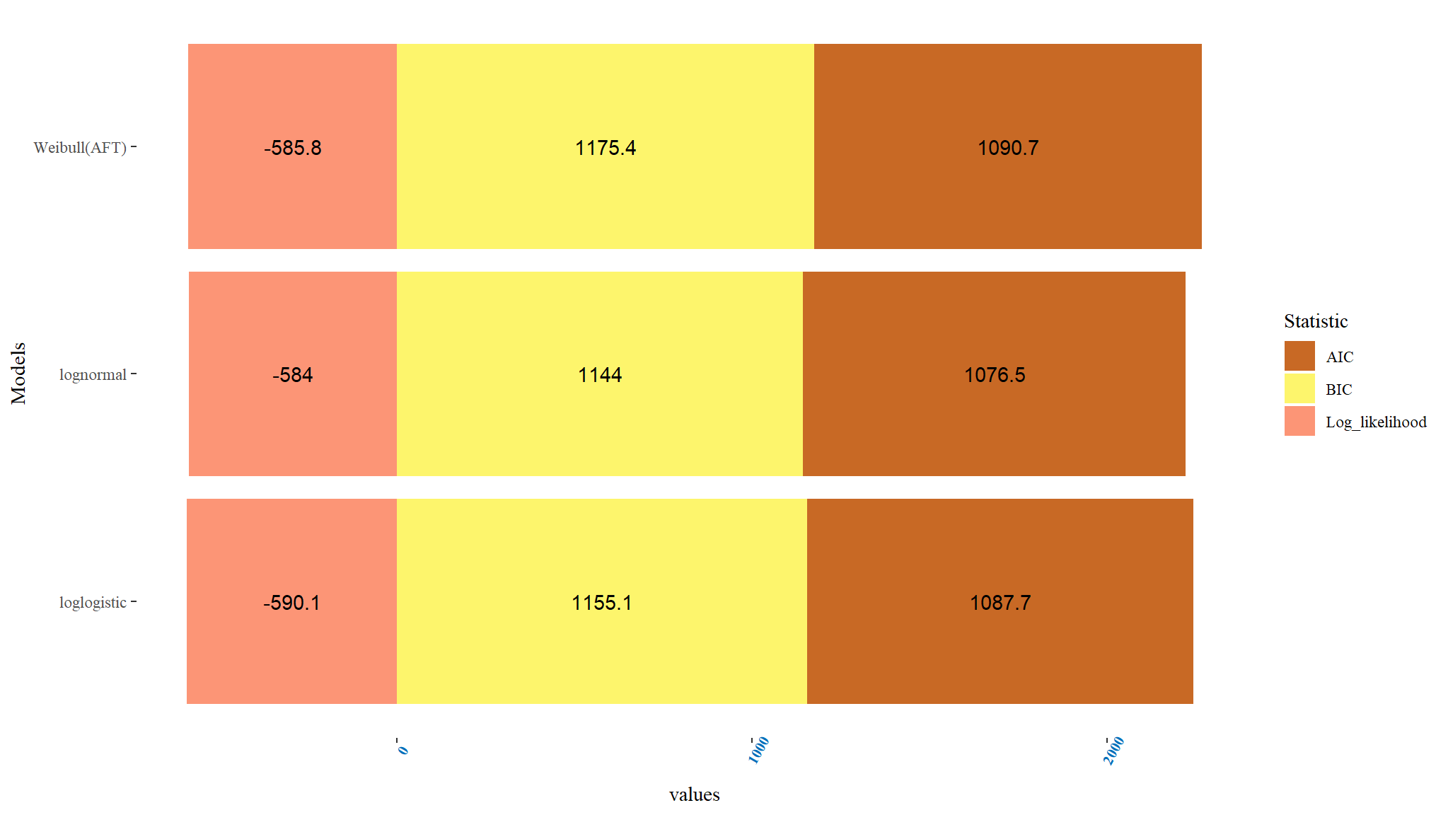
#> Overall p-value 0Comparing Accelerated failure time models
Comments
- When the three accelerated failure time models were weighed and contrasted using AIC, BIC and log likelihood ratio, the one with the smallest value of AIC and BIC were considered the best among the other models.
- From Table above, the Lognormal AFT model can be regarded to be a suitable AFT model for the data since it has the least AIC and BIC values when contrasted with other AFT models. Thus the Lognormal AFT \((AIC=1076.545,BIC=-584.0072)\) was a better fit among all contrasted AFT models.
Compare models graphically
Overal Best Model
- The log-likelihood ratios and AIC were used to choose the model that was overal best for the data.
- Table above displays the log-likelihood ratios and Akaike’s Information Criterion (AIC) for the best PH and AFT models.
- Among the desired models, the best and most efficient model is the one with the lowest AIC value.
- By comparing the AIC values, it was observed that the Lognormal model was the overall best-fitted model for the data.
- Therefore, the data was best fitted using the Lognormal Accelerated Failure Time model.